EXCEL FORMULAS
BASIC EXCEL FORMULAS
1. SUM
The SUM function adds values. You can add explicit numerical values, cell references, ranges, or a mix of all three. The basic syntax is:
SUM(number1, [number2], [number3]...)Note that arguments are separated by commas. A space may also be inserted or may be omitted.
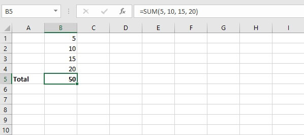
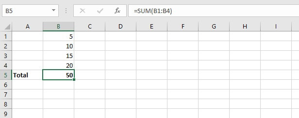
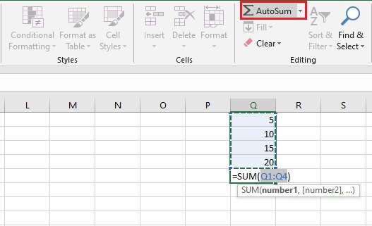
By allowing the use of cell ranges instead of values, you eliminate having to enter each value one by one as you would on a calculator.

2. AVERAGE
Another basic arithmetic calculation that Excel takes care of is the AVERAGE function. As seen before, it eliminates the need to perform a two-step calculation and is, therefore, one of our recommended basic functions.
The syntax of the AVERAGE function is:
AVERAGE(number1, [number2], ….)Arguments may also be entered as a cell range.

3. IF
The IF function ventures into the realm of logical functions. Logical functions basically test whether a situation is true or false. The IF function takes it a step further by performing one action if the situation is true, and another action if it is false. This function is a great example of how Excel can turn a plain data sheet into an analytical tool.
The situation tested may be where one value or statement is equal to, greater than, or less than another value or statement.
The syntax of the IF function is:
IF(logical_test, [value_if_true], [value_if_false])
- Logical_test is the statement to be tested.
- Value_if_true is the value or expression Excel should return if the cell passes the logical test.
- Value_if_false is the value or expression Excel should return if the logical test fails.
In the case of the IF function, if the value_if_true is omitted, the value_if_false must be stated, and vice versa. But both cannot be omitted.
With IF, we can get Excel to perform a different calculation or display a different value depending on the outcome of a logical test. The IF function asks you for the logical test to perform, what action to take if the test is true, and an alternative action if the result of the test is false.
Though both the second and third arguments are declared as optional, at least one of those arguments must be provided.
=IF(B2>=90,“Outstanding”, “”)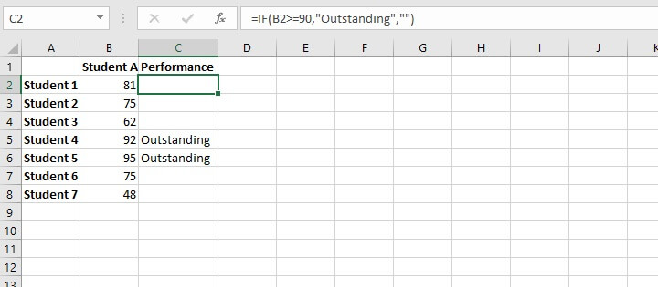
If the value is not greater than or equal to 90, the cell should remain blank (note the empty double quotation marks). This formula is then copied to cells C3 to C8, where C3 evaluates the value in B3, and so on.
To learn more about relative cell references and how they help when copying formulas, check out this resource (Relative References in Excel - A Beginner's Guide).
4. SUMIFS
SUMIFS is a very useful Excel function. It combines the basic SUM operation with an IF logical test to add only cells that meet multiple user-defined criteria.
Up to 127 pairs of criteria may be submitted. Cells that are considered a “match” or “qualifying” would need to satisfy all the stated criteria. SUMIFS is superior to the SUMIF function, which is limited to only one condition being evaluated at a time.
The SUMIFS syntax is:
SUMIFS(sum_range, criteria_range1, criteria1, [criteria_range2], [criteria2],...)
- Sum_range - is the range of cells to sum.
- Criteria_range1 - is the range of cells to be evaluated.
- Criteria1 - is the condition that cells in criteria_range1 must satisfy.
- Criteria_range2 - is the second range of cells to be evaluated.
- Criteria2 - is the condition or criterion that cells in criteria_range2 must satisfy.
All arguments after criteria1 are optional.
Here is an example of SUMIFS at work.
=SUMIFS($C$2:$C$10,$B$2:$B$10,E2)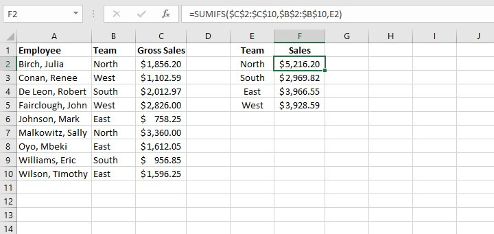
Note the use of absolute cell references above to lock the cell ranges. This prevents shifting of the range when the formula is copied to other cells.
5. COUNTIFS
The COUNTIFS function is another member of the IF family of functions. It counts only cells that satisfy all the stated criteria. COUNTIFS is superior to the COUNTIF function, which allows only one condition to be evaluated at a time.
The syntax of the COUNTIFS function is:
COUNTIFS(criteria_range1, criteria1, [criteria_range2, criteria2]…)
- Criteria_range1 - is the first range to be evaluated.
- Criteria1 - is the first criterion that cells in criteria_range1 must satisfy.
- Criteria_range2 - is the second range to be evaluated.
- Criteria2 - is the first criterion that cells in criteria_range2 must satisfy.
All pairs after criteria1 are optional. Up to 127 range and criteria pairs are allowed.
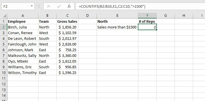
To count the number of sales reps on the North team who achieved more than $1,500 in sales, the formula would be:
=COUNTIFS(B2:B10,E1,C2:C10,E2)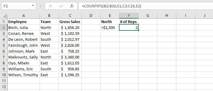
=COUNTIFS(B2:B10,E1,C2:C10,“>1500”)
6. VLOOKUP
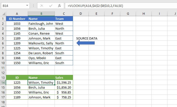
The VLOOKUP function will be a game-changer once you start using it. Use VLOOKUP when you need to find things in a table or an array. VLOOKUP is used in many search-type situations, for example, to find an employee name based on their employee ID.
The VLOOKUP syntax is:
VLOOKUP(lookup_value, table_array, col_index_num, [range_lookup])Here’s what those arguments mean:
- Lookup_value - is what you want to look up.
- Table_array - where you want to look for it.
- Col_index_num - is the column number in the range containing the value to return.
- Range_lookup - type TRUE for an approximate match, or FALSE for exact match.
The formula
=VLOOKUP(A14,$A$2:$B$10,2,FALSE)is entered in cell B14, which returns the name of the employee matching the ID number.
In recent years, VLOOKUP has been outperformed by XLOOKUP, which is more flexible and arguably easier to use. XLOOKUP is available in Microsoft 365 and later.
7. COUNT
The COUNT function will count the number of cells that contain numbers. You can use this function to get the number of entries in a number field that’s in a range or an array of numbers. The syntax of the COUNT function is:
=COUNT(value1, [value2]...)Placing the COUNT function in cell B6 below determines that there are three numeric values between cell B1 and B5.
=COUNT(B1:B5)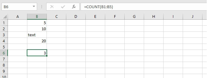

Comments
Post a Comment